


Normalizing Flows in PyTensor#
A hip new algorithm for doing machine learning on distributions is called normalizing flows.
The idea begins with the change of variables formula. We begin with a random variable \(X \sim N(0, 1)\). Suppose we know the PDF for \(X\) (because we do!). What if we instead wanted the PDF for \( Y = \exp(X)\). Do we know that?
The answer is yes! We know it because of the change of variable formula, which states:
Where:
\(g(\cdot)\) is the (unknown!) PDF of the variable \(Y\)
\(f(\cdot)\) if the (known!) PDF of the variable \(X\)
\(G(\cdot)\) is a function with nice properties.
The “nice properties” require (in the most general case) that \(G(x)\) is a \(C^1\) diffeomorphism, which means that it is 1) continuous and differentiable almost everywhere; 2) it is bijective, and 3) its derivaties are also bijective.
A simpler requirement is that \(G(x)\) is continuous, bijective, and monotonic. That will get us 99% of the way there. Hey, \(\exp\) is continuous, bijective, and monotonic – what a coincidence!
Prepare Notebook#
from abc import ABC

import arviz as az
import matplotlib.pyplot as plt
import numpy as np
import preliz as pz
import pymc as pm
from scipy.optimize import minimize

import pytensor
import pytensor.tensor as pt
from pytensor.graph.basic import explicit_graph_inputs
from pytensor.graph.replace import vectorize_graph
from pytensor.graph.rewriting import rewrite_graph
from pytensor.tensor.basic import TensorVariable


plt.style.use("seaborn-v0_8")

%config InlineBackend.figure_format = "retina"
Simple Example: Change of Variables Formula#
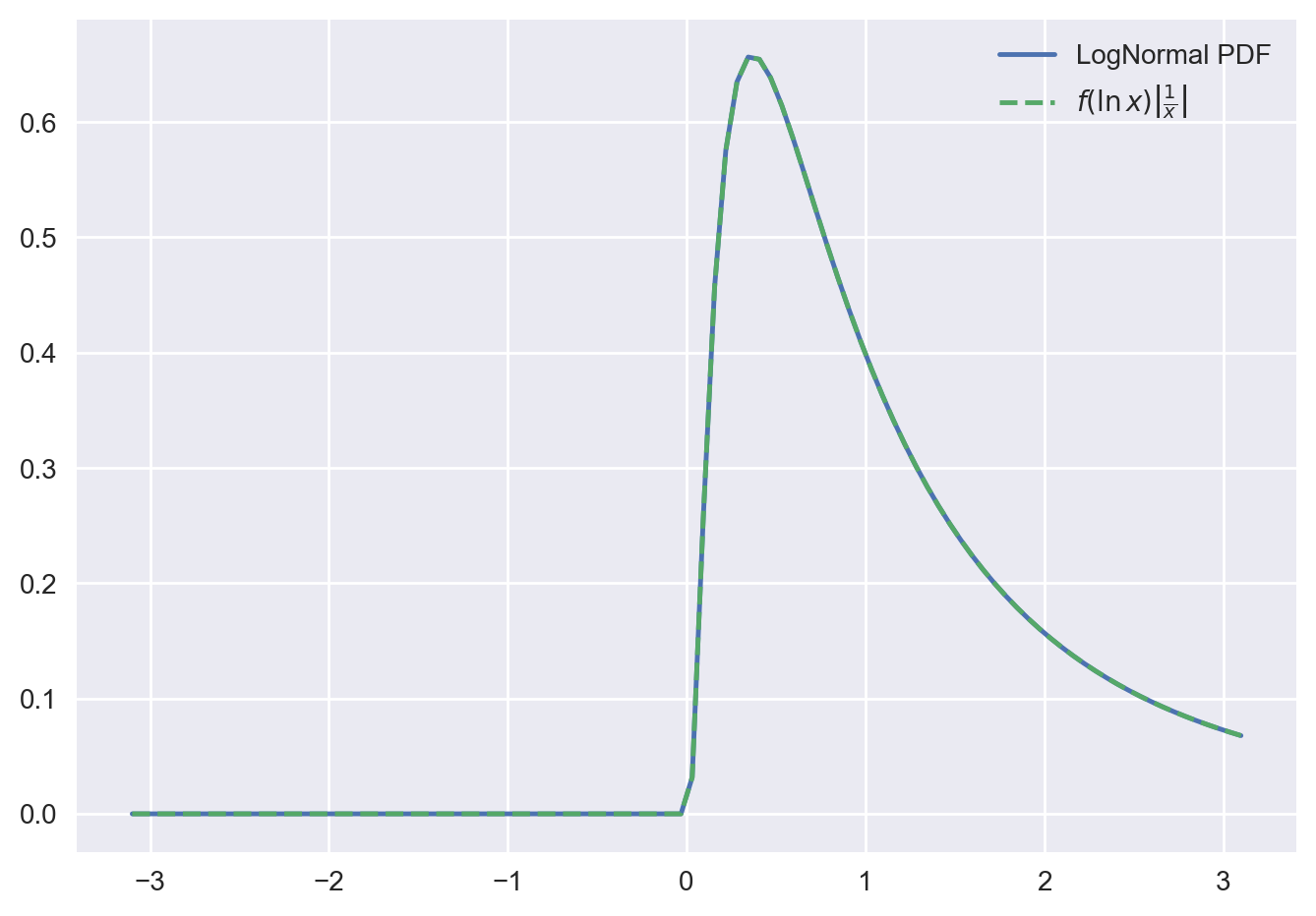
Let’s visualize this result through a concrete example. We look at the transformation of a normal distribution to a lognormal distribution.
X = pz.Normal(0, 1)
Y = pz.LogNormal(0, 1)

x_grid = np.linspace(-3.1, 3.1, 100)

f_values = X.pdf(x_grid)


# This is just a convenient trick: setting the value to 0 if x <= 0
def G_inv(x):
    return np.where(x > 0, np.log(x), 0)


def d_G_inv(x):
    return np.where(x > 0, np.reciprocal(x), 0)


g_values = (X.pdf(G_inv(x_grid))) * np.abs(d_G_inv(x_grid))

fig, ax = plt.subplots()
ax.plot(x_grid, Y.pdf(x_grid), c="C0", label="LogNormal PDF")
ax.plot(
    x_grid, g_values, c="C1", ls="--", label=r"$f(\ln x) \left | \frac{1}{x} \right |$"
)
ax.legend();
/var/folders/wj/wjy2vm8d7_j9v43bv29zcgl80000gq/T/ipykernel_79672/3343765610.py:11: RuntimeWarning: invalid value encountered in log
  return np.where(x > 0, np.log(x), 0)
Normalizing Flows Fundamentals#
In this section, we will explore the core concepts of normalizing flows. along this notebook, we will work one complete example: sampling from a log-normal distribution using normalizing flows.
Before going into the actual example, let us understand the overall strategy.
The change of variables procedure above, is basically all we need to understand normalizing flows. The logic goes like this:
Suppose we have some data \(\mathcal{D} \sim D(\cdot)\), where \(D\) is totally unknown.
We would like to sample from \(D\), which seems hard since we don’t know it.
Instead of sampling from \(D\), let’s instead sample \(F(\cdot)\), where we get to choose \(F\) to be as simple as possible. Say it’s just \(N(0, 1)\)
Then, we’ll use a change of variables to make draws from \(F\) look like draws from \(D\).
We just need a function \(G(x)\) that makes samples \(x \sim N(0, 1)\) look like our data.
\(G\) needs to have the nice properties we want: monotonic, bijective, and invertible. And, we’d like it to have some parameters to learn!
Let’s define a simple base class to represent normalizing flows in PyTensor.
class Flow(ABC):
    __slots__ = ("parameters",)

    def transform(self, x: TensorVariable) -> TensorVariable:
        """Apply function F to the distribution x, along with the jacobian correction"""
        ...

    def inverse_transform(self, x: TensorVariable) -> TensorVariable:
        """Apply inverse function F^{-1} to the distribtuion x"""
        ...
We can now specify two concrete examples:
class Exp(Flow):
    """Exponential transformation"""

    def transform(self, x: TensorVariable) -> TensorVariable:
        return pt.exp(x)

    def inverse_transform(self, x: TensorVariable) -> TensorVariable:
        return pt.log(x)


class Affine(Flow):
    """Affine transformation"""

    __slots__ = ("loc", "scale", "parameters")

    def __init__(self, loc: float = 0.0, scale: float = 1.0) -> None:
        self.loc = pt.as_tensor_variable(loc)
        self.scale = pt.as_tensor_variable(scale)

    def transform(self, x: TensorVariable) -> TensorVariable:
        return self.loc + self.scale * x

    def inverse_transform(self, x: TensorVariable) -> TensorVariable:
        return (x - self.loc) / self.scale
As the composition of two flows is itself a flow, we can define a class that composes them:
def compose(*fns):
    def f(x):
        for fn in fns:
            x = fn(x)
        return x

    return f
Understanding the Forward Pass#
Let’s use these classes to generate a normalizing flow computational graph.
# Random number generation
rng = pytensor.shared(np.random.default_rng(), name="rng")
# Sample from a normal distribution
x = pt.random.normal(0, 1, rng=rng)

# Define the parameters of the affine transformation
loc, scale = pt.dscalars("loc", "scale")
# Define the transformations
transforms = [Affine(loc=loc, scale=scale), Exp()]
# Compose the transformations
flow = compose(*[x.transform for x in transforms])
# Apply the transformations to the random variable
z = flow(x)

# Print the resulting graph
z.dprint()
Exp [id A]
 └─ Add [id B]
    ├─ loc [id C]
    └─ Mul [id D]
       ├─ scale [id E]
       └─ normal_rv{"(),()->()"}.1 [id F]
          ├─ rng [id G]
          ├─ NoneConst{None} [id H]
          ├─ 0 [id I]
          └─ 1 [id J]
<ipykernel.iostream.OutStream at 0x1055e99c0>
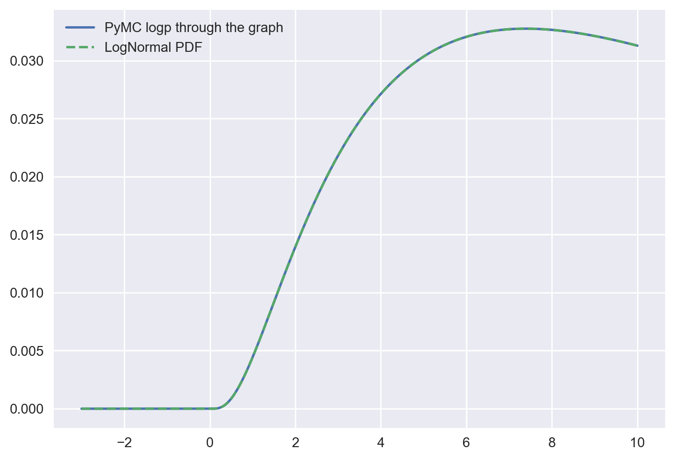
We can now compute the log-density of the transformed variable.
z_values = pt.dvector("z_values")
# The funtion `pm.logp` does the magic!
z_logp = pm.logp(z, z_values, jacobian=True)
# We do this rewrite to make the computation more stable.
rewrite_graph(z_logp).dprint()
Switch [id A] 'z_values_logprob'
 ├─ Isnan [id B]
 │  └─ Mul [id C]
 │     ├─ [-1.] [id D]
 │     └─ Log [id E]
 │        └─ z_values [id F]
 ├─ [-inf] [id G]
 └─ Add [id H]
    ├─ Switch [id I]
    │  ├─ Isnan [id J]
    │  │  └─ Mul [id K]
    │  │     ├─ [-1.] [id D]
    │  │     └─ Log [id L]
    │  │        └─ Abs [id M]
    │  │           └─ Alloc [id N]
    │  │              ├─ scale [id O]
    │  │              └─ Squeeze{axis=0} [id P]
    │  │                 └─ Shape [id Q]
    │  │                    └─ Sub [id R]
    │  │                       ├─ Log [id E]
    │  │                       │  └─ ···
    │  │                       └─ ExpandDims{axis=0} [id S]
    │  │                          └─ loc [id T]
    │  ├─ [-inf] [id G]
    │  └─ Add [id U]
    │     ├─ Check{sigma > 0} [id V]
    │     │  ├─ Add [id W]
    │     │  │  ├─ [-0.91893853] [id X]
    │     │  │  └─ Mul [id Y]
    │     │  │     ├─ [-0.5] [id Z]
    │     │  │     └─ Pow [id BA]
    │     │  │        ├─ True_div [id BB]
    │     │  │        │  ├─ Sub [id R]
    │     │  │        │  │  └─ ···
    │     │  │        │  └─ ExpandDims{axis=0} [id BC]
    │     │  │        │     └─ scale [id O]
    │     │  │        └─ [2] [id BD]
    │     │  └─ True [id BE]
    │     └─ Mul [id K]
    │        └─ ···
    └─ Mul [id C]
       └─ ···
<ipykernel.iostream.OutStream at 0x1055e99c0>
From the log-density graph, we can extract the inputs:
inputs = list(explicit_graph_inputs(z_logp))
inputs
[z_values, scale, loc]
z_values, scale, loc = inputs
We proceed to compile the graph into a function so we can do actual computations.
f_logp_pymc = pytensor.function([z_values, loc, scale], z_logp)
Let’s verify that the resulting log-density of the transformed variable is the same as the log-density of a LogNormal distribution, which is precisely what we expect.
x_grid = np.linspace(-3, 10, 1000)
plt.plot(
    x_grid,
    np.exp(f_logp_pymc(z_values=x_grid, loc=3, scale=1.0)),
    c="C0",
    label="PyMC logp through the graph",
)
plt.plot(
    x_grid,
    pz.LogNormal(mu=3, sigma=1).pdf(x_grid),
    ls="--",
    c="C1",
    label="LogNormal PDF",
)
plt.legend();
Learning the loc and scale parameters#
Suppose now, we just have samples from some “unknown” lognormal distribution, we can learn parameters loc and scale by maximizing the log likelihood of the data
samples = pz.LogNormal(mu=2.234, sigma=0.99354).rvs(5_000)

objective = -pm.logp(z, z_values, jacobian=True).mean()

# We can use pytensor for automatic differentiation
grad_objective = pt.stack(pt.grad(objective, [loc, scale]))
# We compile the graph to make actual computations
f_obj_grad = pytensor.function([z_values, loc, scale], [objective, grad_objective])

# Next, we compute the Hessian matrix
# It would be nicer to just use the hessian function, but pytensor is fussy and doesn't like
# scalar inputs
hess = pt.stack(
    pytensor.gradient.jacobian(
        pt.stack(pt.grad(objective, [loc, scale])), [loc, scale]
    ),
    axis=0,
)

f_hess = pytensor.function([z_values, loc, scale], hess)

f_sample = pm.compile([loc, scale], z)
We can use the scipy.optimize.minimize function to find the maximum likelihood estimates of the loc and scale parameters.
res = minimize(
    lambda x, *args: f_obj_grad(*args, *x),
    jac=True,
    hess=lambda x, *args: f_hess(*args, *x),
    method="Newton-CG",
    x0=[0.8, 0.8],
    args=(samples,),
    tol=1e-12,
)
res
 message: Optimization terminated successfully.
 success: True
  status: 0
     fun: 3.6165369785017196
       x: [ 2.232e+00  9.664e-01]
     nit: 10
     jac: [ 1.643e-13 -4.547e-13]
    nfev: 12
    njev: 12
    nhev: 10
We see that we have recovered the parameters of the lognormal distribution. Let’s compare the samples from the learned distribution with the original samples.
fig, ax = plt.subplots(figsize=(10, 6))
az.plot_kde(
    np.r_[*[f_sample(*res.x) for _ in range(5_000)]],
    plot_kwargs={"c": "C0", "label": "Samples from Learned Distribution"},
    ax=ax,
)
az.plot_kde(
    samples,
    plot_kwargs={"c": "C1", "label": "Samples from Original Distribution"},
    ax=ax,
)
ax.legend(fontsize=12)
ax.set_xlabel("x", fontsize=14)
ax.set_ylabel("Density", fontsize=14)
ax.tick_params(labelsize=12)
ax.set_title(
    "Samples from LogNormal(mu=2.234, sigma=0.99354)", fontsize=18, fontweight="bold"
);
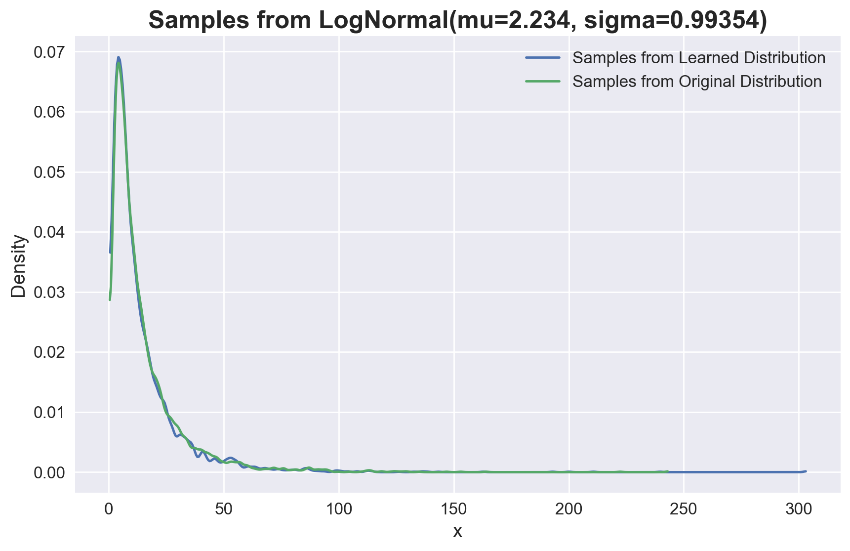
Theese distribution are essentially the same.
Reproducing what PyMC does#
Most of the heavy lifting here was done by PyMC. It already knows how to handle the change-of-variables formula for a wide variety of functions, including \(\exp\) and affine shifts. That’s why things just sort of magically worked up until now.
Recall the formula for change of variables:
Right now in the graph of \(z\), we just have draws from \(x\), passed through the function \(G\). Or:
To get to where we want to go, we need to:
Iterate backwards over all the flows, applying the inverse function to the incoming samples
At the same time, we also need to compute \(\left | \frac{\partial}{\partial x} G^{-1}(x) \right | \) and accumulate their products
We need to get the logp of the original random variable, \(f(x)\), and plug in the result of (1) as the value
Finally, add the log of the product of the determinant corrections.
Since in the end we need the log of the determinant, it will be easier to modify step (2) to accumulate the sum of the log determinant of the transformations
In detail#
We have two transformations, \(H(x) = \exp(x)\) and \(J(x) = a + bx\). Define \(G\) as their composition, \(G \equiv (H \circ J)(x) = \exp(a + bx)\)
For inverses, we have \(H^{-1}(x) = \ln(x)\) and \(J^{-1}(x) = \frac{x - a}{b}\)
So, the inverse of their composition is \(G^{-1} \equiv (J^{-1} \circ H^{-1}) = J^{-1}(H^{-1}(x)) = J^{-1}(\ln(x)) = \frac{\ln(x) - a}{b}\)
For the correction term, we need the determinant of the jacobian. Since \(G\) is a scalar function, this is just the absolutel value of the gradient:
We we will compute \(g(z) = f(\frac{\ln(z) - a}{b}) \left | \frac{1}{b} \cdot \frac{1}{z} \right |\), where \(f(x) = \frac{1}{\sqrt{2\pi}}\exp(-\frac{x^2}{2})\) is a standard normal PDF.
Of course we’ll work with the logp, so we will actually have:
Solution by hand#
We now implement theis analytic procesure in PyTensor:
def standard_normal_logp(x):
    x = pt.as_tensor_variable(x)

    kernel = -(x**2) / 2
    normalizing_constant = -0.5 * pt.log(2 * np.pi)
    return normalizing_constant + kernel
# Get the parameters of the first transform (affine)
loc, scale = transforms[0].loc, transforms[0].scale
z_star = (pt.log(z_values) - loc) / scale
analytic = (
    standard_normal_logp(z_star) - pt.log(pt.abs(scale)) - pt.log(pt.abs(z_values))
)
# Compile the function
f_analytic = pytensor.function([z_values, loc, scale], analytic)
We can pass specific value now and evaluate the analytic function:
f_analytic(samples, loc=3, scale=1)
array([-4.06681489, -3.42976537, -3.42097081, ..., -3.73252572,
       -4.26441774, -3.43616604], shape=(5000,))
We can verify these values are exaclty what we are expecting:
np.testing.assert_almost_equal(
    actual=f_analytic(samples, loc=3, scale=1),
    desired=pz.LogNormal(mu=3, sigma=1).logpdf(samples),
)
Solution using autodiff#
Now we do it again using autodiff. We need the absolute value of the gradient through the whole composite transformation. We do it on a dummy scalar \(x\), then vectorize back up to z_values, since that’s the behavior we want.
We could also do pt.grad(f_inverse(z_values).sum(), z_values), and rely on the fact that the sum function introduces no cross-terms in the gradient expression. This would be the same, but would require you to grok this math fact. We also like that the vectorize way shows off vectorize_graph.
x = pt.dscalar("x")
# Get the inverse of the flows
inverse_flows = [f.inverse_transform for f in reversed(transforms)]

f_inverse = compose(*inverse_flows)
# Use autodiff to compute the log jacobian determinant
log_jac_det = pt.log(pt.abs(pt.grad(f_inverse(x), x)))
# Vectorize the graph
log_jac_det = vectorize_graph(log_jac_det, {x: z_values})

# Compute the logp of the inverse flow
inverse_flow = standard_normal_logp(f_inverse(z_values)) + log_jac_det
# Compile the function
f_logp_flow = pytensor.function(list(explicit_graph_inputs(inverse_flow)), inverse_flow)
As above let’s verify taht the results are consistent and correct:
np.testing.assert_almost_equal(
    actual=f_logp_flow(samples, loc=3, scale=1),
    desired=f_logp_pymc(samples, loc=3, scale=1),
)
Re-do optimization using our new implementation#
Finally, we can re-do the optimization using our new implementation.
objective = -inverse_flow.mean()

grad_objective = pt.stack(pt.grad(objective, [loc, scale]))
f_obj_grad = pytensor.function([z_values, loc, scale], [objective, grad_objective])

hess = pt.stack(
    pytensor.gradient.jacobian(
        pt.stack(pt.grad(objective, [loc, scale])), [loc, scale]
    ),
    axis=0,
)
f_hess = pytensor.function([z_values, loc, scale], hess)
res = minimize(
    lambda x, *args: f_obj_grad(*args, *x),
    jac=True,
    hess=lambda x, *args: f_hess(*args, *x),
    method="Newton-CG",
    x0=[0.8, 0.8],
    args=(samples,),
    tol=1e-12,
)
res
 message: Optimization terminated successfully.
 success: True
  status: 0
     fun: 3.616536978501722
       x: [ 2.232e+00  9.664e-01]
     nit: 10
     jac: [ 1.643e-13 -4.357e-13]
    nfev: 12
    njev: 12
    nhev: 10
We get the expected results 🚀!
References#
Watermark#
%load_ext watermark
%watermark -n -u -v -iv -w -p pytensor
Last updated: Sun Aug 17 2025

Python implementation: CPython
Python version       : 3.12.11
IPython version      : 9.4.0

pytensor: 2.31.7

numpy     : 2.2.6
pytensor  : 2.31.7
arviz     : 0.22.0
preliz    : 0.20.0
pymc      : 5.25.1
scipy     : 1.16.1
matplotlib: 3.10.5

Watermark: 2.5.0
License notice#
All the notebooks in this example gallery are provided under a 3-Clause BSD License which allows modification, and redistribution for any use provided the copyright and license notices are preserved.
Citing Pytensor Examples#
To cite this notebook, please use the suggested citation below.
Important
Many notebooks are adapted from other sources: blogs, books… In such cases you should cite the original source as well.
Also remember to cite the relevant libraries used by your code.
Here is an example citation template in bibtex:
@incollection{citekey,
  author    = "<notebook authors, see above>",
  title     = "<notebook title>",
  editor    = "Pytensor Team",
  booktitle = "Pytensor Examples",
}
which once rendered could look like: